
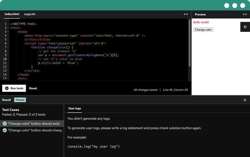
This course includes our updated coding exercises so you can practice your skills as you learn.
See a demo
Master time series analysis and forecasting with python, covering exponential smoothing and cutting-edge models like LinkedIn, Silver Kite, Prophet, and Amazon Cronos for real-world predictions.
Explore version one of the time series assistant, review its architecture and core functionalities, and learn its capabilities and limits for time series analysis.
Diogo introduces his analytics-focused background, including management science and data-driven business work, and invites you to connect, learn, and apply insights from a restaurant analytics startup.
Stay ahead with a constantly updated course on time series analysis and forecasting in Python, as this 2026 edition updates content and invites your feedback to improve the learning experience.
Master time series analysis and forecasting in Python by exploring data, identifying seasonality, and applying models from exponential smoothing to ARIMA, while practicing with real data and a capstone project.
Learn to turn raw time series data into insight using Python, with real data, real questions, and real decisions, by slicing data, spotting patterns, and testing ideas.
Learn to load a time series dataset with pandas, inspect the dataframe, explore state holiday values using value counts, and binarize holidays to a 0/1 indicator in Colab.
Learn to explore retail data by counting stores, subsampling ten stores with a fixed random state, and compute mean sales per store, then identify each store's all-time high day.
Standardize weekday sales with z-scores to enable apples-to-apples store comparisons. Group by store and day of week and analyze mean standardized sales to reveal Sunday seasonality and other patterns.
Filter the data for day seven and visualize store sales with matplotlib. Notice Sundays can introduce noise in standardization.
Remove day-of-week seven observations for store 353 to clean the data, then standardize sales by store and analyze intra-week seasonality with a visual intro-week plot.
Analyze the impact of promotions by comparing average sales on promotion days versus non promotion days, then compute per store promo uplift and identify top and bottom performers.
Explore time series data with Python, learn to spot patterns and trends, and turn numbers and dates into visual stories. Preview forecasting concepts with real-world examples and simple, hands-on coding.
Explore time series data with the Bitcoin daily price dataset (2014–2023) to reveal volatility, trends, autocorrelation, and seasonality for forecasting and real-world applications, including weather forecasting and economics.
Set up Python in Google Colab, mount Google Drive, import pandas and matplotlib, load bitcoin price data, and preview the first rows to prepare for time series analysis.
Master the time series index by converting dates to date-time objects and setting them as the dataframe index, using pandas, matplotlib, and statsmodels for efficient analysis, plotting, and resampling.
learn to use exploratory data analysis to understand time series by computing seven-day rolling averages, plotting close prices, and performing monthly resampling for mean and index max.
Compute percentage changes of closing prices with pandas to derive daily returns and reveal volatility. Identify days with more than 10% change using absolute values, noting the 97 volatile days.
Learn to enhance data visualization by adding titles and plotting daily closing price with a 30-day rolling volume on a dual-axis chart to reveal correlations.
Learn practical data manipulation for time series: identify missing values, apply backward and forward fill, interpolate, and compute 7-day closing averages and 30-day rolling volume with pandas.
Explore time series feature engineering by extracting date features from the index, year, month, day, day of week, weekend, and add lagged variables for forecasting.
Learn seasonal decomposition of time series into trend, seasonality, and error terms. Distinguish additive from multiplicative seasonality using visualization and model performance in Python.
Visualize seasonality in time series using month plots and quarter plots from Statsmodels, compare actual monthly values to their averages, and explore resampled monthly data.
Examine seasonal decomposition of a time series by separating trend, seasonal cycles, and noise, using seasonal decompose for monthly data with period 12 and additive or multiplicative seasonality.
Explore autocorrelation by comparing a time series with its lagged values to reveal how past information helps predict the future.
Explore autocorrelation and partial autocorrelation with statsmodels, visualizing lagged relationships in time series data. Interpret these plots to understand information added by specific lags and seasonal patterns for future forecasting.
Explore the partial autocorrelation function (pacf) to isolate direct relationships between current values and past observations, removing intermediate effects, and contrast with the autocorrelation function.
Analyze partial autocorrelation with Python using Bitcoin adjusted close to reveal that the day before holds unique information. Learn to identify informative lags with pacf and relate them to acf.
Build a reusable time series analysis script that streamlines data cleaning, indexing dates, exploratory data analysis, visualization, and autocorrelation analysis, serving as a practical template for forecasting workflows.
Explore time series forecasting of stock prices by modeling errors with relevant regressors, assessing data relevance, and understanding external factors like events, economic conditions, and sentiment.
Review how we transformed raw time series data into stories by analyzing trends, applying Python libraries, and visualizing seasonality and autocorrelation to forecast stock prices.
Analyze how forecasts miss the mark through cases like fidget spinners, LTCM, Google Flu Trends, and the Hindenburg omen, and learn the limits of models.
Load the department sales data into a pandas DataFrame, parse and format dates, set the date index, and configure weekly frequency to ready the data for time series analysis.
Plot the weekly sales from the data frame, set a title and figure size, and mark holidays with vertical red dashed lines to reveal their relationship to sales.
Conduct exploratory data analysis on weekly sales using acf and pacf with 60 lags and perform multiplicative seasonal decomposition with a 52-week period to reveal trend, seasonality, and residuals.
Learn exponential smoothing and Holt-Winters in Python, covering simple, double, and triple methods through a case study, measure forecast errors, handle weekly vs daily data, and assess pros and cons.
Explore a Telco Wave case study to forecast weekly customer complaints, analyze data and hidden patterns, and align the workforce with customer needs to reduce complaints and boost profits.
Set up exponential smoothing with holt-winters, prep weekly customer complaints data, rename the series to y, clean commas, convert to integer, and plot to reveal trend and multiplicative seasonality.
Analyze seasonality in weekly data, resample to monthly with month end, and assess multiplicative versus additive seasonal models using Holt-Winters, guided by autocorrelation insights.
Split time series data into training and test sets by removing the last periods and using an 80/20 split for unbiased evaluation, with two to three training periods.
Split the time series into training and test sets for a 13-week horizon, select the usable Y, and apply simple double and triple exponential smoothing against the business goal.
Explore how simple exponential smoothing blends the current level with recent observations via alpha to forecast and smooth spikes in time series data.
Explore simple exponential smoothing with statsmodels to forecast time series by updating the level using a smoothing coefficient, fitting to training data, and generating forecasts.
Apply double exponential smoothing to capture both level and trend in sales data. Use alpha and beta to weight recent data and trend changes, noting no seasonality.
Build a double exponential smoothing model in Python to predict and visualize time series, using statsmodels with additive trend and no seasonality.
Explore triple exponential smoothing, aka Holt-Winters, for time series with level, trend, and seasonality. Learn how alpha, beta, and gamma weight the components to improve forecasting and handle seasonal patterns.
Apply Holt-Winters triple exponential smoothing with multiplicative seasonality to forecast time series weekly data, using a 52-week seasonal period and evaluate forecast errors in Python.
Learn to measure forecast accuracy with mean absolute error, RMSE, and MAPE. Explore their tradeoffs, including interpretability, outlier handling, and when to compute them in Python.
Analyze model outcomes by computing RMSE, MAE, and MAPE using sklearn.metrics, comparing true versus predicted values, and formatting results in a reusable model assessment function for time series evaluation.
Learn to predict the future with a Holt-Winters model. Compare additive and multiplicative seasonality, tune parameters, test on 13-week forecasts, and plot training data against the forecast.
Load bitcoin price data and prepare daily data with a date index and adjusted close. Fit a Holt-Winters model, test seasonal periods of 7 and 365, and discuss crypto volatility.
Extend our useful time series template by adding libraries, renaming the series to Y, adjusting frequency, and building reusable functions, including model assessment, for flexible Colab workflows.
Explore Holt-Winters, a simple forecast method for trend and seasonality that relies on recent data with level, trend, and seasonal components, but supports only one seasonal factor and no regressors.
Study the capstone air miles time series by setting monthly frequency, visualizing data, forecasting the next 12 months with holt-winters, and evaluating errors with MAE, RMSE, and MAPE.
Learn to prepare monthly time series data in Python, visualize trends and seasonality, perform multiplicative seasonal decomposition, assess ACF and PACF, and set up training and test sets.
Complete task three: set the last 12 months as the test set and the training data. Build the Holt-Winters time series model with exponential smoothing and multiplicative seasonality.
Learn to forecast 12 periods with an exponential smoothing (holt-winters) model, assess accuracy with metrics, visualize training, test, and future predictions, and explore EDA and frequency as building blocks.
Explore the foundational ARIMA, SARIMA, and SARIMAX models and their use in time series forecasting. Apply cross-validation, parameter tuning, and external factors in real-world data examples with statsmodels.
Forecast daily revenues for a chocolate shop using past sales data to uncover patterns, seasonal trends, and holidays, then plan inventory and staffing with ARIMA models and external regressors.
Set up the arima workflow in python, preprocess data, parse dates, and configure daily frequency. Explore seasonality and autocorrelation to guide data-driven parameter selection, with multiplicative decomposition insights.
Explore the autoregressive component of Arima, where the past values and lagged data predict the future, with examples like coffee consumption and chocolate revenues.
Explore the integrated component of ARIMA by applying differencing to convert nonstationary data into stationary signals, and learn how the augmented Dickey-Fuller test checks stationarity to improve predictions.
Assess stationarity with the augmented Dickey-Fuller test, interpret the p-value against 0.05 for the null of a unit root, and apply differencing to obtain a stationary time series.
The moving average component of ARIMA learns from previous prediction errors to smooth data, adapt quickly to recent changes, and improve forecasts by incorporating past mistakes.
Explore ARIMA modeling in python with a train–test split, nonseasonal order, and forecasting using endogenous and exogenous inputs like discount and coupon rates for 30 days.
Explore ARIMA in practice: use past values t-1, t-2, t-3, a constant, and forecasting errors with differencing and a rolling forecasting approach, building toward sarima.
Explore SARIMA, building on ARIMA, by adding a seasonal component to capture seasonality, using PDQ and seasonal m to separate seasonal and non-seasonal data for cleaner forecasts.
Build a sarima model, select initial parameters, and test seasonal orders (7 and 365 days). Assess predictions and model performance, noting computational limits and the potential of external variables.
Explore how SARIMA combines ARIMA components, seasonal lags at t-7 and t-14, and past forecast errors to generate a final forecast.
Master time series analysis with SARIMAX, which combines SARIMA with exogenous variables to incorporate external factors like temperature and holidays for better forecasts.
Learn SARIMAX with exogenous regressors, clean data by removing percentage symbols, and forecast using discount rate and coupon rate. Emphasize cross-validation and parameter tuning.
Explore building a sarimax-style forecast by combining non-seasonal arima components, seasonal terms, and exogenous variables like discount and coupon, resulting in a six-component forecast; then master cross-validation and parameter tuning.
Master cross-validation for time series by testing across different seasonalities with rolling and sliding forecasts. Extend and trim training data to build robust forecasts and assess model performance.
Learn to implement time series cross-validation with a time series split, set up train and test windows (last 30 days), apply ARIMAX, and evaluate with RMSE, MAE, and Mop.
Tune parameters to maximize forecast accuracy by systematically testing autoregressive models with different lags, using a reusable template and automated error tracking in Python.
Explore parameter tuning for time series models by building an eight-combination parameter grid, applying time-series cross-validation with RMSE, and optimizing forecasting performance.
Explore parameter tuning for time series analysis using grid search and cross validation with sarima models (p, d, q), compute rmse, and store results for robust forecasting.
Explore parameter tuning results for a time series model by transforming the RMSE grid into a data frame, identifying the best params, and preparing for future forecasting with lagged features.
Discover how to handle future data in time series forecasting by identifying future regressors, coordinating with finance and marketing teams, and building exogenous inputs for models like N-Beats and TFT.
Isolate the target and features, load and format future regressors, apply best parameters, adjust units by multiplying by 100, and prepare to predict future discount and coupon rates.
Build and tune a sarimax model, perform cross-validation and parameter tuning, fit and print the summary, then generate future predictions and plot the results.
Explore SARIMAX pros and cons, compare Holt-Winters, and use the PMD removal library for quick cross-validation, noting short-term strength, long-term limits, and single seasonality.
Master modern time series forecasting with Prophet and Silver Kite. Set up the Python environment, model seasonality and holidays, and tune parameters for accurate forecasts.
Forecast bike rental demand with Prophet and Python through a hands-on bike-sharing case study. Prepare data, perform eda, engineer features, tune parameters, and visualize insights.
Explore structural time series by decomposing data into trend, seasonality, exogenous regressors, and an error term, then use Prophet with dynamic holidays and built-in cross-validation for practical forecasting.
Analyze bike sharing demand using a rich Washington DC dataset from 2011–2012, exploring temperature, weather, date, and city events to forecast demand with practical, profit-oriented models.
Load data and prepare a Prophet-based time series workflow in Google Colaboratory, using numpy, pandas, and matplotlib to model daily bike sharing counts with a parameter grid.
Renames variables and formats dates, converts the weather situation into categorical dummies with get_dummies and drop first, and drops unused columns to streamline the data frame for time series analysis.
Perform exploratory data analysis in Python using a code template to set the date stamp as the index. Observe trend and multiplicative seasonality, plus spikes and autocorrelation and partial autocorrelation.
Model dynamic holidays like Valentine's Day by capturing event-driven demand with a lower window of minus three days and an upper window of one day after, using profit.
Engineer holiday features in Python with pandas, building a holidays dataframe for general holidays, Christmas, New Year's, and Easter, and ensure consistent date handling for profit modeling.
Explore Prophet model parameters, including multiple seasonalities (yearly, weekly, daily), multiplicative or additive seasonality, holidays, and priors for seasonality, holidays, and trend to balance overfitting and underfitting.
Learn to build a Prophet model, configure yearly and weekly seasonality, and add regressors such as holidays and weather features to improve forecasts.
Explore how prophet's regressor coefficients address non-linearity and multicollinearity, interpret coefficients with a ChatGPT-assisted function, distinguishing multiplicative versus additive effects in weather-related predictors.
Apply cross validation to the model by building a data frame cross-validation, configuring period, horizon, and initial settings, and running in parallel to assess forecasting performance.
Analyze cross-validated forecast outputs, examine prediction intervals and actuals across horizons, and evaluate performance with RMSE and the map while plotting metrics to diagnose data issues.
Identify spikes in residuals, inspect metrics, and fix the data by replacing oct 29–30, 2012 with oct 28’s values to stabilize rmse and map before feature engineering.
Explore feature engineering for time series by creating lagged temperature features (lags 1, 3, 5, 7), assessing their correlation with demand, and selecting a single lag to improve model performance.
Define a parameter grid for time series models, including change point prior scale, seasonality and holidays priors, and seasonality mode; generate all parameter combinations and prepare for tuning.
Build a parameter tuning pipeline in Python for time series models using cross validation and RMSE as the error metric.
Create a pandas dataframe of all parameters, evaluate tuning results, and select the best additive seasonality configuration to guide future predictions.
Learn to build a Python-based time series forecasting workflow, preparing data, engineering features like holidays and lag, tuning the model, predicting the future, and visualizing results.
Build a tuned Prophet model by cleaning the training data, removing NaNs, and training only the last 30 days using the best parameters to forecast future values.
Learn practical python time series forecasting by building a 30-day future data frame, incorporating future regressors, and producing a forecast with yhat and the upper and lower values.
Visualize time series forecasts with Prophet in Python using ChatGPT-assisted code. Explore components, holidays, weekly and yearly seasonality, and regressors with interactive Plotly visuals and actual versus forecast.
Assess Prophet's flexibility, built-in visualization and cross-validation, and its handling of non-linearity and multicollinearity, while noting slower optimization and poor short-term dynamics for sudden changes.
Updates September 2025:
All the Darts library sections were re-recorded.
New sections on Intermittent Time Series and Classification for Time Series.
New Projects!
More Concise videos by coding with GenAI.
Updates August 2025:
New AI Course Assistant is live!
Updates July 2025:
Fully updated the exercises in the section Python Essentials.
Updates March 2025:
Google TSMixer Launched
Introduction to Time Series Analysis and Exponential Smoothing Python tutorials remade.
Updates December 2024:
Amazon AutoGluon launched
Library requirements.txt file for all sections added
Updates October 2024:
Amazon Chronos launched
N-BEATS launched
Updates September 2024:
TFT and TFT Capstone Project added
Updates August 2024:
Course remade 100%
Silverkite, LSTM and Projects added
Welcome to the most exciting online course about Forecasting Models in Python.
I will show you everything you need to know to understand the now and predict the future.
Forecasting is always sexy.
Knowing what will happen usually drops jaws and earns admiration.
On top, it is fundamental in the business world. Companies always provide Revenue growth and EBIT estimates, which are based on forecasts.
Who is doing them?
Well, that could be you!
WHY SHOULD YOU ENROLL IN THIS COURSE?
Master the Intuition Behind Forecasting Models
No need to get bogged down in complex math.
This course emphasizes understanding the why behind each model. We simplify concepts with clear explanations, intuitive visuals, and real-world examples—focusing on what really matters so you can apply these techniques confidently.
Comprehensive Coverage of Cutting-Edge Techniques
You’ll dive deep into the most advanced and sought-after time series forecasting methods that are crucial in today’s data-driven world:
Exponential Smoothing & Holt-Winters – Handle trends and seasonality with elegance.
Advanced ARIMA Models (SARIMA & SARIMAX) – Incorporate external variables for enhanced forecasts.
Facebook Prophet – Robust, high-accuracy forecasts with minimal data prep.
Temporal Fusion Transformers (TFT) – State-of-the-art deep learning for multiple time series.
LinkedIn Silverkite – Flexible, powerful forecasting across contexts.
N-BEATS – Cutting-edge neural networks for diverse forecasting challenges.
GenAI with Amazon Chronos – Discover how generative AI is revolutionizing forecasting.
Google TSMixer (NEW) – Leverage Google’s breakthrough architecture for time series.
Amazon AutoGluon (NEW) – Automate high-performance forecasting pipelines.
Intermittent Time Series (NEW) – Tackle irregular, sporadic patterns with specialized techniques.
Classification for Time Series (NEW) – Expand beyond forecasting into predictive categorization.
Code Python Together, Line by Line
We’ll code side by side, ensuring you understand every step.
From data preparation to model implementation, you’ll learn how to write and refine each line of Python code needed to master these forecasting techniques.
Practice, Practice, Practice
Each lesson includes hands-on challenges and case studies, from sales to demand forecasting
You’ll apply what you’ve learned to real datasets, solve real-world problems, and solidify your skills through practical application.
Are You Ready to Predict the Future?
Did I spike your interest? Join me and learn how to predict the future!