Your cart is empty.
Keep shopping

Teach on Udemy
Turn what you know into an opportunity and reach millions around the world.
Learn MoreLinear Algebra for Data Science and Machine Learning using R
Rating: 4.8 out of 54.8(7 ratings)
74 students
Linear Algebra for Data Science and Machine Learning using R
Vectors, Matrices, Solving Linear Equations, Factorization, Eigenvectors, Least Squares, SVD
Created bySyed Mohiuddin
Last updated 11/2025
English
English [Auto],
What you'll learn
- Fundamentals of Linear Algebra
- Applications of Matrices, Vectors and operations on Matrices and Vectors with implementation in R
- Solve Systems of Linear Equations and implementation in R
- Matrix Factorization and implementation in R
- Computation of Eigenvalues, Eigenvectors and Eigen Decomposition with their implementation in R
- Solving Least Squares problems
- Singular Value Decomposition with its implementation in R
Explore related topics
Coding Exercises
This course includes our updated coding exercises so you can practice your skills as you learn.
See a demo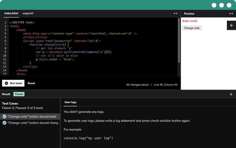
Course content
19 sections • 160 lectures • 9h 45m total length
- What you are going to learn in this course2:47
Learn linear algebra for data science and machine learning using R, covering vectors, matrices, determinants, inverses, norms, eigenvalues, eigenvectors, singular value decomposition, and practical R code demos.
- Introduction1:47
Explore how linear algebra underpins data science and machine learning, and master concepts like vectors, matrices, and tensors, and the rules to manipulate them for machine learning and deep learning.
- What is Linear Algebra?1:10
Explore how linear algebra powers data science by representing data as vectors, matrices, and tensors. See how matrices organize rows as samples and columns as attributes via linear equations.
- Why Linear Algebra?0:56
Learn linear algebra to preprocess data, transform it, and visualize in higher dimensions. This foundation underpins machine learning and deep learning, supports regression, optimization, classification, dimensionality reduction, and neural networks.
- Installing R Software4:34
Download R from CRAN using Linux, macOS, or Windows. Complete the setup with defaults, create a desktop shortcut, and open the R GUI console; next, learn about installing R Studio.
- Installing RStudio3:12
Install RStudio, the integrated development environment for writing and executing R scripts, after ensuring R is installed, then download the desktop installer from the RStudio website and follow on-screen steps.
- Look around RStudio Interface9:07
Navigate the RStudio interface, an integrated development environment for R, to write and run code in the text editor, view results in the console, and manage the working directory.
- Help & Examples Facility for R Features and Functions2:51
Learn to use the built-in help and examples in the official R documentation. Access help.start, the help function, and the question mark, and view examples for functions like sum.
- Changing Look and Feel of RStudio1:40
Explore customizing the RStudio look and feel through global options, adjusting appearance, font size, and editor theme, and set the default working directory—optional and not obstructing command execution.
- Some General Functions Good to Know4:33
Explore essential R functions for development, including get to display current working directory and set the working directory to a path, and ls, rm, library, and history to manage objects.
- Writing R Program using RGui4:14
Write and run your first R program using the R GUI or RStudio; print hello R and save your work as a script for multi-statement programs.
- Writing R Program using RStudio4:21
Set the working directory in RStudio, create an R script, write print statements to display hello R in the console, save as first.r, and remember R is case sensitive.
- Using Comments in R Scripts1:37
Discover how to document R scripts with hash comments, how the interpreter ignores them, and how to efficiently comment multiple lines using one hash per line.
- Scalars and Vectors7:42
Learn scalars and vectors, including magnitude and components; a vector is a one dimensional array of real numbers in rn. Understand column and row representations for data science.
- Vectors
- Vectors in 2-Dimensional Space4:32
Explore two-dimensional vectors in R2, arrows from the origin to (2,4) and (-3,5) showing direction and magnitude. Represent vectors as ordered numbers with column form used in data science.
- Vectors
- Vectors in 3-Dimensional Space2:41
Explore vectors in three dimensional space with three components plotted from the origin along x, y, and z axes, including column and row representations and data science vectors.
- Vectors with n-Components3:20
Represent data in n-dimensional space with vectors of n components in r^n, using column vectors to handle higher dimensions and align attributes across cities like London and Paris.
- R Code - Creating Vectors12:35
Create vectors in R with c and assign, view contents, and measure length to handle n-dimensional data. Explore London, Paris, and Lisbon weather vectors as examples.
- Creating Vectors
- Practice #1
- R Code - Create Vectors using Sequence Operator & Function9:25
Create vectors of consecutive numbers in R using the colon operator or sequence function, with ranges and by steps such as 1 to 6 and 6 to 1.
- Creating Vectors using Sequence
- R Code - Accessing & Modifying Vectors7:24
learn to access and modify vectors in r using one-based indexing with square brackets, handle out-of-range values as na, and apply relational operations to set elements to zero.
- Accessing & Modifying Vectors
- Zero and Ones Vectors2:04
Explore zero vectors as the origin in R2, R3, and RN, and learn that a ones vector has all components equal to one, denoted by 1_n for n components.
- Zero and Ones Vectors
- R Code - Zero and Ones Vector4:20
Learn to create zero and ones vectors in R using the c function, rep function, and vector function, with three- and eight-component examples in numeric and integer types.
- Zero and Ones Vectors
- Quiz Solutions0:03
- Vector Addition4:16
Explore vector addition by adding corresponding components of column vectors, illustrated with family income and expenses, and extend to u plus v in R2, R3, and RN.
- R Code - Vector Addition3:33
Demonstrates vector addition through element wise addition of corresponding components of two vectors, with examples h and w, and u and v, yielding (14000, 9000) and (9, -3, 7).
- Vector Addition
- Scalar Multiplication4:55
Explore scalar multiplication, applying a scalar to each vector component to produce a new vector; see how income and expenses examples illustrate length scaling with positive and negative scalars.
- R Code - Scalar Multiplication4:14
Demonstrate scalar multiplication by multiplying each vector component by a scalar to form a vector; illustrate element-wise results with income 8000 and expenses 5000, and vector u [3, -7, 5].
- Scalar Multiplication
- Vector Properties2:45
Explore the vector properties in n-dimensional space, including commutative and associative vector addition, the existence of a zero vector, and distributive and scalar-multiplication laws for vectors.
- Vector Properties
- Linear Combinations of Vectors2:05
Learn how addition and scalar multiplication form linear combinations of vectors, illustrated by 2u plus 3v, and generalize to v1 through vn with scalars c1 through cn.
- R Code - Linear Combinations of Vectors2:00
Demonstrate forming linear combinations by adding scaled vectors in R, using u = (3, -7) and v = (6, 4) to produce (24, -2) elementwise.
- Linear Combination
- Vector Transpose2:19
Learn how column vectors store data, such as weather for London and Paris, and how transposing converts between column and row with the superscript t, returning to the original vector.
- R Code - Vector Transpose1:22
Learn how to transpose a vector in R using the t function, turning a column vector into a row vector and vice versa, demonstrated with vector L.
- Vector Transpose
- Dot Product or Inner Product5:56
Explore the dot product, or inner product, of vectors, showing how u^T v yields a scalar that measures alignment and direction in R^n, with examples in R^2 and R^3.
- R Code - Dot Product6:54
Compute the dot product of two vectors in R using %*% or crossprod, producing a scalar; ensure equal dimensions and view examples like (2,4) and (-3,5) yielding 14.
- Dot Product
- Outer Product7:18
Learn how the outer product forms an n by n matrix by multiplying a column vector by the transpose of another vector, with examples in R2 and R3.
- R Code - Outer Product4:45
Explore outer product of two vectors in R using t cross prod, producing a matrix; see examples with u=(2,4), v=(-3,5) and u=(3,-2,5), v=(6,4,2).
- Outer Product
- Quiz Solutions0:03
- Matrices - Context of Data Science4:10
Understand how matrices store tabular data in data science, with six observations and seven attributes, using row and column indices to reference elements in a two-dimensional array.
- Martrices
- Dimension or Size4:23
Explore how matrices define dimension by rows and columns, with square, rectangular, wide, and tall examples, diagonal elements, and links to linear equations in data science and machine learning.
- R Code - Creating Matrices5:53
Create matrices in R with the matrix function and c to input elements, show column-wise and row-wise options, and set dimensions with nrow, ncol, or dim; retrieve diagonals with diag.
- R Code - Matrix Functions1:55
Explore how to determine a matrix’s dimensions and size in R using dim, nrow, ncol, and length on a 3-by-2 matrix, revealing rows, columns, and total elements.
- Matrices
- R Code - Naming Rows and Columns of Matrix3:12
Assign names to matrix rows and columns in R using rownames and colnames, turning indices into April, July, October and into max temperature and min temperature.
- R Code - Accessing and Modifying Elements of Matrix3:42
Learn to access and modify matrix elements in R using row-column indexing with square brackets, starting from one, and single-position indexing for column-wise storage.
- R Code - Appending Rows and Columns4:24
Learn to append rows and columns to a matrix in R using rbind and cbind, and assign the results back to the matrix M.
- R Code - Deleting Rows and Columns of Matrix3:10
Shows how to delete rows and columns in a three-by-three matrix in R using negative indexing, including removing the second row and the third column by reassigning the matrix.
- R Code - Creating Matrix using rbind() and cbind()2:53
Explore creating matrices in R with rbind and cbind to bind rows and columns from vectors like April, July, and October, yielding matrix M.
- Matrix Transpose4:41
Explore the matrix transpose, swapping rows and columns to form A^T, with examples A and B, and learn that a transpose of a transpose returns the original matrix.
- R Code - Matrix Transpose2:18
Learn to transpose a matrix in R using t, interchanging rows and columns; a 3x2 matrix becomes a 2x3, and the transpose of a transpose returns the original matrix.
- Matrix Transpose
- Symmetric Matrix4:25
Explore why a symmetric matrix equals its transpose and must be square, illustrated with A and A^T. See how distance matrices demonstrate symmetry and why B and rectangular C fail.
- R Code - Symmetric Matrix5:23
Demonstrate how to determine whether a matrix is symmetric in R by computing the transpose with t and comparing the matrix to its transpose, using examples of varying dimensions.
- Symmetric Matrices
- Identity Matrices1:42
Explore identity matrices as square matrices with ones on the diagonal and zeros elsewhere, denoted I, and see that multiplying any matrix by I yields the original matrix.
- R Code - Identity Matrices2:55
Learn to create identity matrices in R with the Dag function for two by two, three by three, and five by five sizes, with diagonal elements one and zeros elsewhere.
- Identity Matices
- Diagonal Matrix2:00
Explore diagonal matrices, square matrices with nonzero diagonal elements and zero off-diagonal elements. Identity matrices are diagonal, and diagonal matrices can be rectangular as well.
- R Code - Diagonal Matrix4:12
Explore creating diagonal matrices in R using the Dag and Diag functions, set diagonal values and retrieve diagonal elements, while non-diagonal entries remain zero.
- Diagonal Matrices
- Triangular Matrix1:37
Explore upper and lower triangular matrices in linear algebra for data science and machine learning using R, where the diagonal and entries above or below it determine zeros and nonzeros.
- Triangular Matrix
- Zero and Ones Matrix2:04
Explore zero and ones matrices, defining a zero matrix as all-zero elements and a ones matrix as all-one elements, with examples across various dimensions.
- R Code - Zero and Ones Matrix2:43
Learn to create zero and ones matrices in R using the matrix function, specifying rows and columns to form three by three and other dimensions.
- Zero and Ones Matrix
- Quiz Solutions0:03
- Matrix Addition5:32
Learn to perform matrix addition element-wise, preserving dimensions, as shown with two by two and two by three matrices where corresponding elements are summed.
- R Code - Matrix Addition2:50
Perform matrix addition by adding corresponding elements of two matrices of the same dimension, illustrated with a 2x3 example and specific element-wise sums.
- Matrix Addition
- Scalar Multiplication4:12
Learn scalar multiplication of matrices by multiplying each element by a scalar. The result preserves dimensions, with examples on 2x2 and 2x3 matrices.
- R Code - Scalar Multiplication2:05
Learn how to perform element-wise scalar multiplication on matrices in R, multiplying each entry by a scalar to yield a matrix of the same dimensions.
- Scalar Multiplication
- Hadamard Product5:38
Perform the Hadamard product, or element-wise product, by multiplying corresponding elements of two matrices with identical dimensions, as shown with A and B (2x3); the result preserves the same shape.
- R Code - Hadamard Product2:51
Learn to perform the Hadamard product by multiplying corresponding elements of two matrices of the same dimensions, as shown with a 2x3 example.
- Hadamard Product
- Trace of Matrix2:39
Compute the trace by summing a matrix's diagonal elements to yield a scalar; 2×2 and 3×3 use A11, A22, A33, while 2×3 uses A11 and A22, aiding eigenvalue verification.
- R Code - Trace of Matrix3:03
Compute the trace of a matrix in R by summing diagonal elements to yield a scalar, using the pragma package with library(pragma) and trace, noting non-square matrices trigger an error.
- Matrix Trace
- Matrix Multiplication5:21
Master matrix multiplication, not elementwise like addition, and dot product rule. Ensure A is m by p and B is p by n to yield an m by n result.
- R Code - Matrix Multiplication3:14
Demonstrate matrix multiplication in R by computing the dot product of A's rows with B's columns, ensuring A's columns equal B's rows and using %*%.
- Matrix Multiplication
- Properties of Matrix Operations4:09
Learn the algebraic properties of matrix operations, including commutative and associative matrix addition, scalar distribution, noncommutative multiplication, identity matrices, left and right distributivity, and transpose rules.
- Matrix Power1:23
Compute the powers of a matrix by multiplying A by itself k times, preserving n by n dimensions, with examples such as a two by two matrix.
- R Code - Matrix Power4:00
Compute the matrix power in R by multiplying a square matrix by itself k times using the matrix gal package and the matrix.power function.
- Matrix Power
- Diagonal Matrix Multiplication6:04
Multiplying a diagonal matrix by a matrix scales each row of the second matrix by the corresponding diagonal element, as shown in a 3x3 example.
- R Code - Diagonal Matrix Multiplication4:55
Show how diagonal matrix multiplication in R scales the rows of B by A’s diagonal elements, and how B is scaled by A when reversed.
- Quiz Solutions0:03
- Determinants7:37
Explore determinants as a map from square matrices to real numbers, computed via two-by-two and three-by-three submatrices, cofactors, and checkerboard signs, with examples and notes on singular matrices.
- R Code - Determinants4:35
Compute determinants of square matrices in R using the det function, illustrated with 2x2 and 3x3 examples, showing determinants can be negative or zero.
- Determinants
- Properties of Determinants1:15
Explore the core determinant properties: det(I)=1; det(A^T)=det(A); det(AB)=det(A)det(B); det(A^n)=det(A)^n; and det(A)=1/det(A^{-1}), enabling easier work with complex matrix operations.
- Determinants
- Inverse of Matrix4:01
Explore the inverse of a matrix, its relationship to the identity matrix, and conditions for existence in square matrices using determinants; learn methods like Gaussian elimination.
- R Code - Matrix Inverse3:18
compute the inverse of a square matrix in R using the solve function, with 2x2 and 3x3 examples.
- Matrix Inverse
- Singular and Invertible Matrices1:10
Learn how the determinant governs invertibility: a non-zero determinant makes a matrix invertible (non-singular), while a zero determinant yields a singular, non-invertible matrix.
- R Code - Singular Matrices4:17
Explore checking matrix singularity and invertibility in R by determinants and the Matrix Calc package; use is.singular.matrix and det, and compute inverses with solve when possible.
- Singular Matrix
- Properties of Inverse1:54
Explain the key properties of matrix inverses, including left and right inverses, inverse of a product, inverse of an inverse, and the relation with transpose.
- Properties of Inverse
- Quiz Solutions0:03
- System of Linear Equations6:41
Apply linear algebra to data science and machine learning by studying systems of linear equations, represented with matrices and vectors, and distinguish linear relationships using coefficients, variables, and constants.
- Systems of Linear Equations
- Types of Systems3:20
Explore systems of linear equations, where a system uses the same variables and yields a unique solution, infinitely many solutions, or no solution, visualized as intersecting, coinciding, or parallel lines.
- Matrix Notation2:55
Represent systems of linear equations with matrices by forming the coefficient matrix and appending the right-hand side as an augmented matrix. Use two- and three-variable examples to illustrate.
- Matrix Notation
- Elementary Row Operations6:40
Explore elementary row operations—interchange, scaling, and replacement—and how they modify augmented matrices without changing the underlying linear system, and see that these operations are reversible for solving.
- Gauss Elimination Method9:40
Learn to solve linear systems using the Gaussian elimination method on augmented matrices, turning them into row echelon form with pivot elements, and perform back substitution.
- Gauss Elimination Method
- Gauss-Jordan Elimination Method7:00
Apply Gauss-Jordan elimination to the augmented matrix to obtain row reduced echelon form, turning pivots into zeros above and below, and solve the linear system.
- R Code - Gauss Jordan Elimination Method5:00
Demonstrates Gauss-Jordan elimination in R by converting an augmented 3x3 matrix to reduced row echelon form to solve for x1, x2, x3 using the rref function.
- Gauss-Jordan Elimination Method
- Quiz Solutions0:03
- Matrix Vector Product Ax=b5:25
Represent a linear system as a matrix vector product ax=b, where A is m-by-n, x is the variables vector, and b is the constants.
- Matrix Vector Product
- Systems of Equations as Linear Combinations4:32
Represent systems of linear equations as a matrix-vector product A x = b and as a linear combination of A's columns, illustrating how coefficients and unknowns form b.
- Classification of Matrix Vector Product4:21
Examine the matrix vector product ax=b, with A as the coefficient matrix and x as variables, classifying by m vs n cases, yielding unique solution, multiple solutions, or no solution.
- Solving Systems of Linear Equations using Matrix Inverse5:23
Represent a system of linear equations as A x = b and solve with the matrix inverse, requiring a square, invertible A (nonzero determinant), illustrated with a two-equation example.
- R Code - Solving Systems of Linear Equations using Matrix Inverse6:10
solve systems of linear equations in R by constructing matrix A and vector b, then compute x as A inverse times b using the solve function, with two- and three-variable examples.
- Solving Systems of Linear Equations using Matrix Inverse
- Solving Systems of Linear Equations using Cramer's Rule4:21
Learn how to solve a system of linear equations using Cramer's rule with a square invertible matrix, calculating determinants and replacing columns to find x1 and x2.
- R Code - Solving Systems of Linear Equations using Cramer's Rule6:14
Solve a two-equation system using Cramer's rule in R by forming matrix A of coefficients and vector b, computing determinants, and obtaining x1 and x2 as 8 and -3.
- Solving Systems of Linear Equations using Cramer's Rule
- R Code - Solving Systems of Linear Equations using qrSolve() function6:17
Solve systems of linear equations in R with qrSolve() from the pragma package by building matrix a and vector b; show x1=8, x2=-3, and x1=3, x2=5, x3=-1 for three-equation case.
- Solving Systems of Linear Equations
- Quiz Solutions0:03
- Lengths and Norms2:10
Explore vector length through norms, including L2 (Euclidean), L1 (Manhattan), p norms, and the max norm, and compare their behavior with outliers and sparsity.
- L2 Norm4:00
Compute vector length with the L2 norm, or Euclidean distance, by taking the square root of the sum of squared components. For example, (3,4) yields 5.
- R Code - L2 Norm4:15
Compute the L2 norm (Euclidean length) of vectors in R using the pragma package and the norm function, with examples for v = c(3,4) and w = c(3,-2,5).
- L1 Norm2:35
Compute the L1 norm, or Manhattan distance, by summing the absolute values of a vector's components, from R2 to R3 and beyond.
- R Code - L1 Norm3:15
Compute the L1 norm (Manhattan distance) of vectors in R using the pragma package and the norm function with type 1, illustrated with vectors (3,4) and (3,-2,5).
- LP Norm2:15
Compute the LP norm for a vector, a generalization of L1 and L2, by taking the p-th root of the sum of absolute values to the p power.
- R Code - LP Norm2:39
Learn to compute the LP norm of vectors in R, a generalization of L1 and L2, using the norm function with p = 4 and the pragma package.
- L-Infinity Norm2:22
Compute the l infinity norm, or max norm, of a vector by taking the maximum of the absolute values of its components.
- R Code - L Infinity Norm2:30
Compute the l infinity norm of a vector in R by taking the maximum of its absolute components, using the norm function with Inf and library(pragma) to load the package.
- Norms
- Quiz Solutions0:03
Requirements
- You should have familiarity with fundamentals of Maths
- All the implementation of Linear Algebra concepts are in R, so familiarity with R will be an added advantage
Description
This course will help you in understanding of the Linear Algebra and math’s behind Data Science and Machine Learning. Linear Algebra is the fundamental part of Data Science and Machine Learning. This course consists of lessons on each topic of Linear Algebra + the code or implementation of the Linear Algebra concepts or topics.
There’re tons of topics in this course. To begin the course:
We have a discussion on what is Linear Algebra and Why we need Linear Algebra
Then we move on to Getting Started with R, where you will learn all about how to setup the R environment, so that it’s easy for you to have a hands-on experience.
Then we get to the essence of this course;
Vectors & Operations on Vectors
Matrices & Operations on Matrices
Determinant and Inverse
Solving Systems of Linear Equations
Norms & Basis Vectors
Linear Independence
Matrix Factorization
Orthogonality
Eigenvalues and Eigenvectors
Singular Value Decomposition (SVD)
Again, in each of these sections you will find R code demos and solved problems apart from the theoretical concepts of Linear Algebra.
You will also learn how to use the R's pracma, matrixcalc library which contains numerous functions for matrix computations and solving Linear Algebric problems.
So, let’s get started….
Who this course is for:
- Anyone who is curious about how Linear Algebra is used in Machine Learning
- Anyone who wants to understand Maths and Linear Algebra behind Data Science
- Anyone who wants to develop fundamental foundations for deployment of Machine Learning Techniques